Simulating deformation of fibrin clot with ANSYS

In the same spirit as my last post, which is an almost verbatim transcript of a poster I presented at Swarthmore College, this post is a reproduction of the final report I wrote for a solid mechanics course, originally titled “E59 Project: Simulating deformation of fibrin clot using ANSYS.”

Abstract

A 3D printed scale model of a blood clot was mapped. Nodal coordinates, along with empirically determined material properties, were entered into ANSYS (Release 17.2). The model was simulated using ANSYS Beam4 elements, and solved for nodal displacements in the x, y and z-directions. These displacements were subsequently used to calculate stress and strain and the bulk Young’s moduli of the clot: E_x, E_y and E_z. Results are summarised in table 1.

Ex (Pa)	Ey (Pa)	Ez (Pa)
113.5	109.1	16.17

Table 1: Young's moduli.

All three moduli fell within the range 0.1–1500 MPa obtained from past literature. E_x and E_y matched each other closely, with a percentage difference of 4%, supporting the assumption of isotropy in a fibrin clot. E_z deviated from E_x and E_y by close to 90%. This discrepancy could most likely be attributed to the small sample size, the injection of the clot into a microscope slide chamber during its preparation, and limitations of optical scanning under a confocal microscope. Overall, results showed that 3D printing a scale model and simulating the deformation of a fibrin clot in ANSYS is a viable method for modelling clot mechanical behaviour, although to extend this procedure to more complex clots, automation of some steps would be essential.

Introduction

Blood clots—made predominantly of a material called fibrin—that form within a patient’s blood vessels can lead to adverse conditions such as ischaemic stroke and myocardial infarction. Traditionally treatment for such blood clots—called thrombi—involves administering a clot-dissolving chemical agent to the patient; the drug travels in the bloodstream and affects the body systemically. This could be fatal, if the patient has other benign blood clots that also become dissolved by the drug.

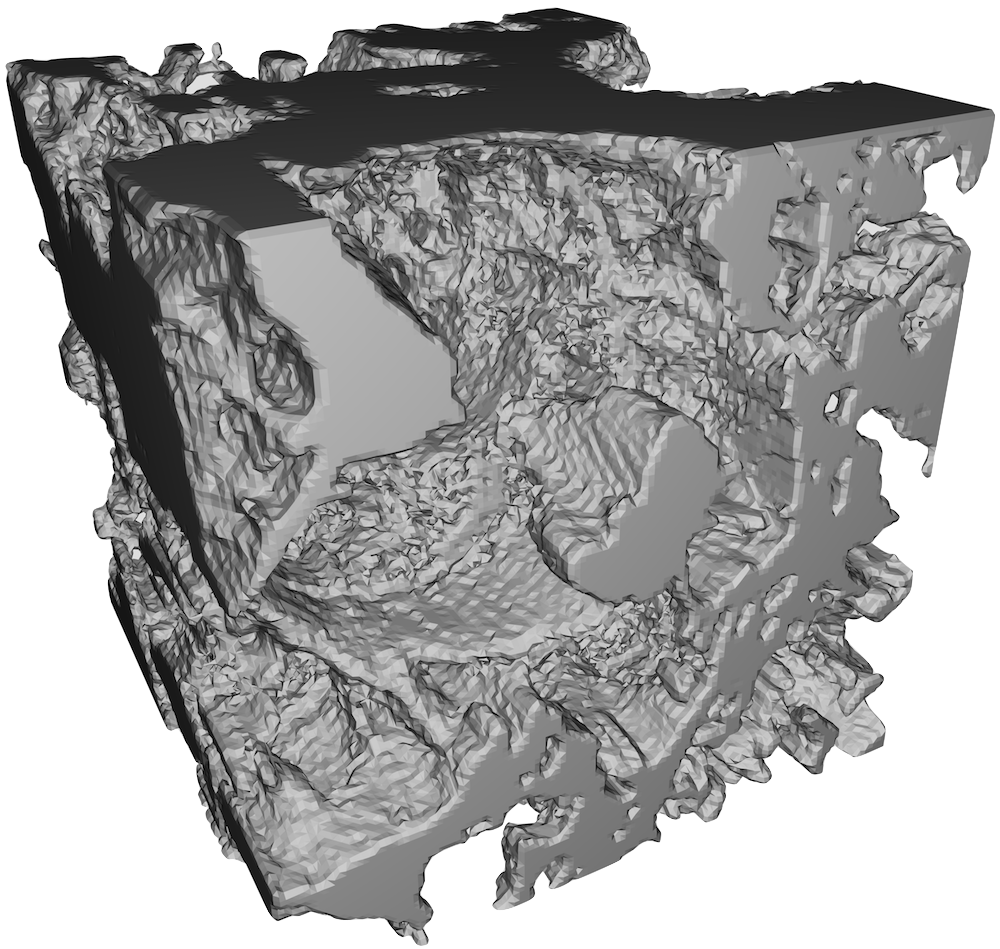
Sonothrombolysis—the dissolution of blood clots using a combination of ultrasound and violently cavitating microbubbles—aims to circumvent this issue by breaking down blood clots through mechanical force. To understand more fully the interactions between mechanical force and networks of fibrin, I fabricated in the summer of 2016 a blood clot from 1.5 mg/mL purified fibrinogen, 4% Alexa Fluor 488 fluorescent dye, 3 mM CaCl₂ and 0.1 unit/mL thrombin, then imaged it under a confocal microscope and reconstructed its structure in 3D for visualisation on a computer, as shown in figure 1. As purified fibrinogen rather than blood plasma was used, the clot was made up exclusively of fibrin, free from blood cells, platelets or other components normally present in human blood.

Figure 1: 3D visualisation of the fibrin clot modelled.

The goal of this project was to model the deformation of this clot under load, using ANSYS [1]. One of the most important characteristics of a material is its Young’s modulus E. Although the Young’s modulus and Poisson’s ratio ν of an individual fibrin fibril must be found empirically, once their values were obtained from past literature, I used ANSYS to simulate the clot under axial loading in order to find its bulk Young’s modulus (as distinguished from the Young’s modulus of an individual fibril) in each of the three spatial dimensions, i.e. E_x, E_y and E_z. Empirical measurements of the modulus of an aggregate clot also exist [2], placing its value between 1 and 15,000 dyne/cm², or between 0.1 and 1,500 Pa, so a comparison was made between the simulated Young’s moduli and the empirical measurements. Although the Poisson’s ratio of the aggregate clot is also important, no empirical value was available for comparison, so I did not attempt to find it from simulation.

Theory

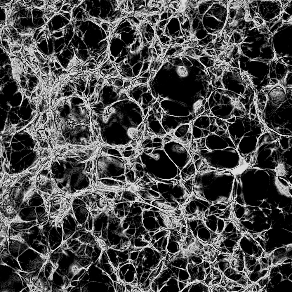
There are two types of ANSYS elements available to model a fibrin clot: solid elements and beam elements. Beam elements are the more suitable choice here, given that most fibrin fibrils are rope-shaped (see figure 2).

Figure 2: Composite confocal micrograph of the fibrin clot modelled. The thick clumps in figure 1 are due to a combination of factors, including the limited resolution of the confocal microscope, and noise.

It is therefore convenient to model these fibrin ‘ropes’ as cylindrical beam elements of constant cross-sectional area. Interconnections between ropes will be modelled as ANSYS nodes; the interconnecting ropes themselves will be modelled as beams, or ‘sticks’. Figure 3 is a picture of what such a ‘stick’ model might look like. Curved fibrils can be modelled as a series of shorter straight beams, connected by intermediate nodes.

Figure 3: The beam or ‘stick’ model. Since the beams are flexible, another description might be the spring model, the implications of which are explored more fully in the Discussion.

The 3D ANSYS beam element Beam4, a schematic of which is shown in figure 4, offers six degrees of freedom: displacement u_x, u_y, u_z and rotation R_x, R_y, R_z [3]. It is an elastic element, capable of axial, torsional and flexural loadings [1]. There are six parameters that need to be specified to fully define this beam element.

Figure 4: Beam4 3D element [1].

For a circular cross section of radius r, they are [4]:

1. cross-sectional area $A = \pi r^2$
2. second moment of area about the z-axis $I_z = \frac{1}{4}\pi r^4$
3. second moment of area about the y-axis $I_y = I_z$
4. thickness of cross section in the z-direction $t_z = 2r$
5. thickness of cross section in the y-direction $t_y = t_z$
6. polar moment of inertia $J_x = \frac{1}{2}\pi r^4$.

When the clot is subjected to an axial force $N$, the stress is given by $\sigma = N/A$, where $A$ is the cross-sectional area of the clot sample. The corresponding strain is given by $\epsilon = \Delta L/L$, where $L$ is the length of the clot sample along a particular axis, and $\Delta L$ is the change in this length as the clot is strained. The Young’s modulus can then be calculated from the equation

$$\begin{equation} E = \frac{\sigma}{\epsilon} \end{equation}$$

along each axis. Note that since $A$ is the cross-sectional area of the sample as if it were solidly filled with fibrin, the true cross-sectional area—which is the sum of the cross-sections of the fibrils only—is smaller. As a result, the true stress and true Young’s modulus will be larger. In other words, the predicted Young’s modulus of my model is a lower bound for the true value. Denser clots made from a higher concentration of thrombin have less empty space between the fibrin fibrils, so the lower bound will be closer to the true value; denser clots are however exponentially more complex to model.

The question of what boundary conditions to use is best answered by considering actual conditions in a thrombus. A thrombus partially or completely closes the blood vessel it resides in, so its boundary is the vascular wall. Although the vascular wall is also flexible, it deforms much less than the fibrin in the clot itself. The boundary can effectively be considered immobile relative to any deformations of the fibrin clot, so I will use fixed supports in my simulation.

Procedure

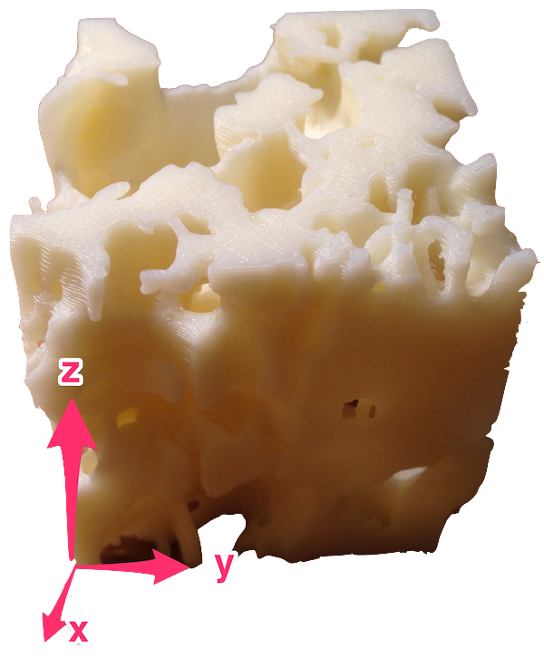
As mentioned, ANSYS Beam4 elements are straight, so each of the fibrin fibrils—which were curved—was approximated by a series of short, straight elements of uniform circular cross section. Nodes along each fibril were identified, their coordinates measured by hand using a ruler on a 3D printed scale model of the clot. The coordinate space is shown in figure 5.

Figure 5: Coordinate space. The actual clot sample had a depth (x) of 48.46 microns, width (y) of 48.46 microns, and height (z) of 50.48 microns. In the scale model, the width and depth were 4.8 cm, the height was 5.0 cm.

Once all nodes were catalogued, they were entered in a .txt file.

Material properties were specified: Young’s modulus $E = 5 \times 10^6$ Pa [5] and Poisson’s ratio $\nu = 0.4999999$ [6]. In reality $\nu$ of fibrin may exceed 0.5, but ANSYS linear material models do not allow for $\nu > 0.5$. In practice this is of little concern, as there was ample room between the fibrin fibrils that they would not come into contact with each other, even with the volume expansion predicted by $\nu > 0.5$. Note that the bulk modulus $K$ given by

$$\begin{equation} K = \frac{E}{3(1-2\nu)} \end{equation}$$

implies that $\lim_{\nu\rightarrow0.5} K$ does not exist, hence the choice of $\nu = 0.4999999$.

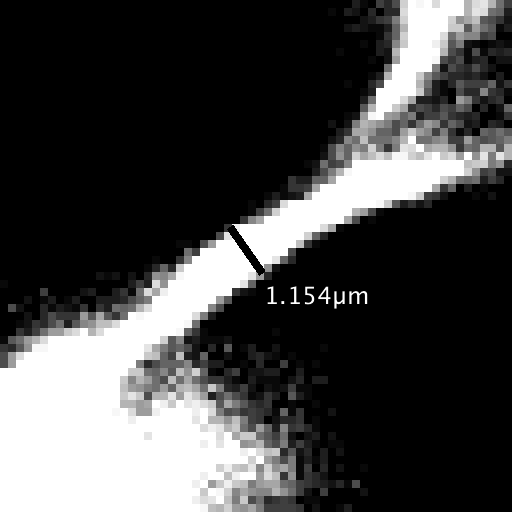
The diameter $d = 2r$ of individual fibrils was measured using the programme Fiji [7] to be $1.154 \times 10^{−6}$ m (see figure 6).

Figure 6: Diameter of fibril.

The corresponding ANSYS element parameters were calculated and entered into the .txt file:

1. $A = 1.046 \times 10^{−12}$ m²
2. $I_z = 8.71 \times 10^{−26}$ m⁴
3. $I_y = I_z$
4. $t_z = 1.154\times 10^{−6}$ m
5. $t_y = t_z$
6. $J_x = 1.741\times 10^{−25}$ m⁴.

With the clot model fully defined in ANSYS, the model was loaded in the x, y and z directions, one direction at a time. To load it in the x direction for instance, all nodes present on the negative x-plane were fixed; a force of $1\times 10^{−9}$ / no. of nodes, was applied to each node present on the positive x-plane. The y and z planes were each loaded separately in a similar manner.

Once ANSYS solves the model for each set of loading and support conditions, nodal displacements for the loaded nodes (on the positive plane) were recorded and averaged. These values were used to find the Young’s moduli E_x, E_y and E_z.

Results

Calculating E_x

Figure 7 shows the clot model loaded on the positive x-plane.

Figure 7: Simulation of axial loading on x-plane.

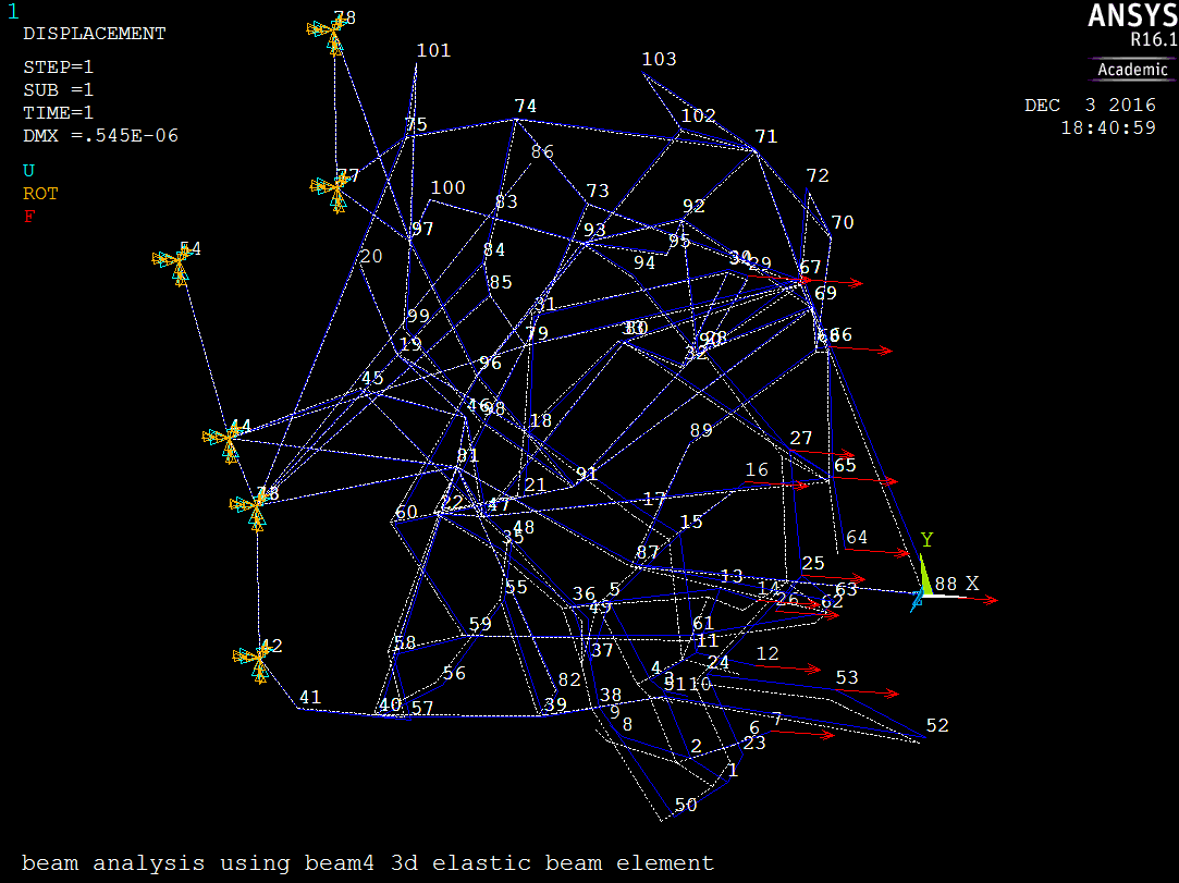
The average x-displacement of all positive x-plane nodes was

$$\eqalign{ \bar{u}_x &=& (0.2256 + 0.2225 + 0.18154 + 0.13528 + 0.2567 + 0.5446 \\ && + 0.16003 + 0.05249 + 0.08709 + 0.15954 + 0.09805 + 0.03807 \\ && − 0.007380 + 0.2903)/14 \\ &=& 0.17462\times 10^{−6}~\text{m.}}$$

Strain was $\epsilon_x = \frac{0.17462}{48.46} = 3.603\times 10^{−3}.$

Stress was $\sigma_x = \frac{1\times 10^{-9}}{(48.46\times 10^{-6})(50.48\times 10^{-6})} = 0.4088~\text{Pa.}$

The Young’s modulus was $E_x = \frac{\sigma_x}{\epsilon_x} = 113.5~\text{Pa.}$

Calculating E_y

Figure 8 shows the clot model loaded on the positive y-plane.

Figure 8: Simulation of axial loading on y-plane.

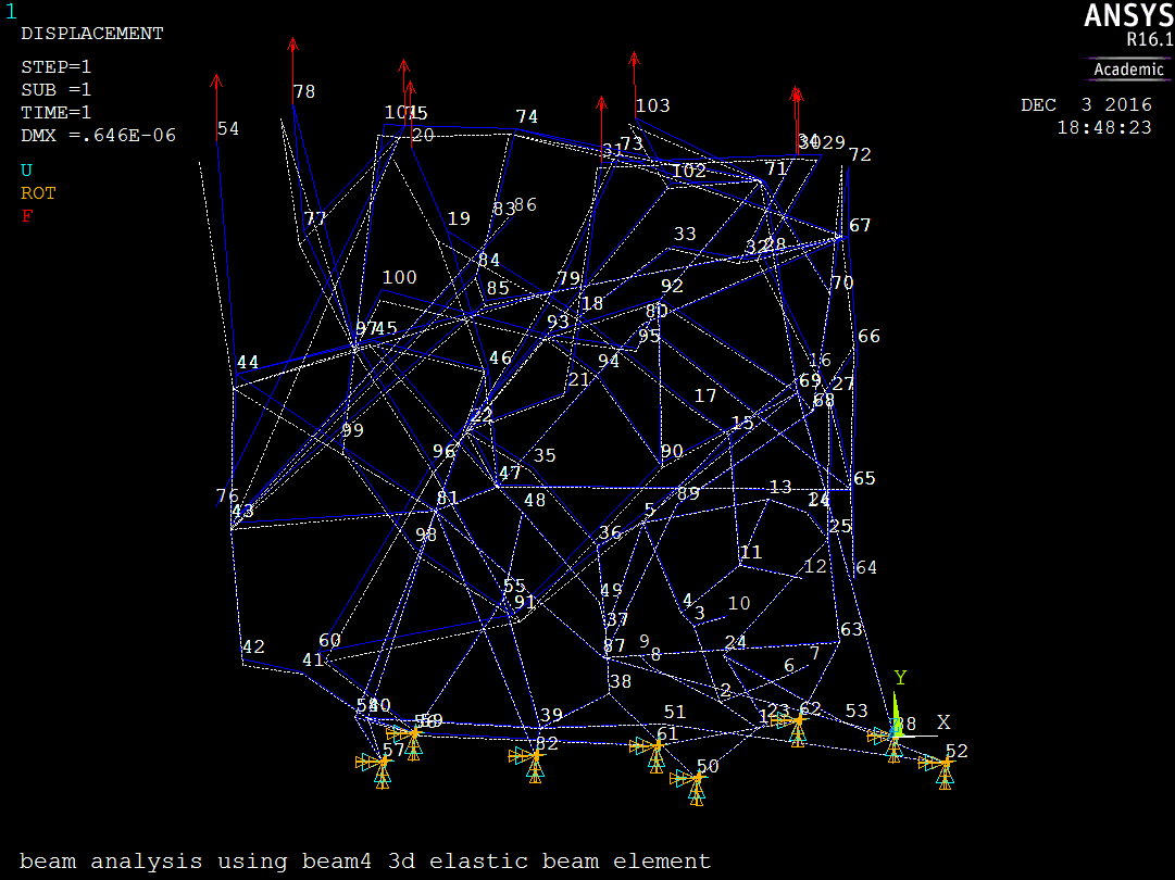
The average y-displacement of all positive y-plane nodes was

$$\eqalign{ \bar{u}_y &=& (0.2262 + 0.07960 + 0.08479 + 0.10736 + 0.3379 + 0.2209 \\ && + 0.2755 + 0.12051)/8 \\ &=& 0.18160\times 10^{−6}~\text{m.}}$$

Strain was $\epsilon_y = \frac{0.18160}{48.46} = 3.747\times 10^{−3}.$

Stress was $\sigma_y = \frac{1\times 10^{-9}}{(48.46\times 10^{-6})(50.48\times 10^{-6})} = 0.4088~\text{Pa.}$

The Young’s modulus was $E_y = \frac{\sigma_y}{\epsilon_y} = 109.1~\text{Pa.}$

Calculating E_z

Figure 9 shows the clot model loaded on the positive z-plane.

Figure 9: Simulation of axial loading on z-plane.

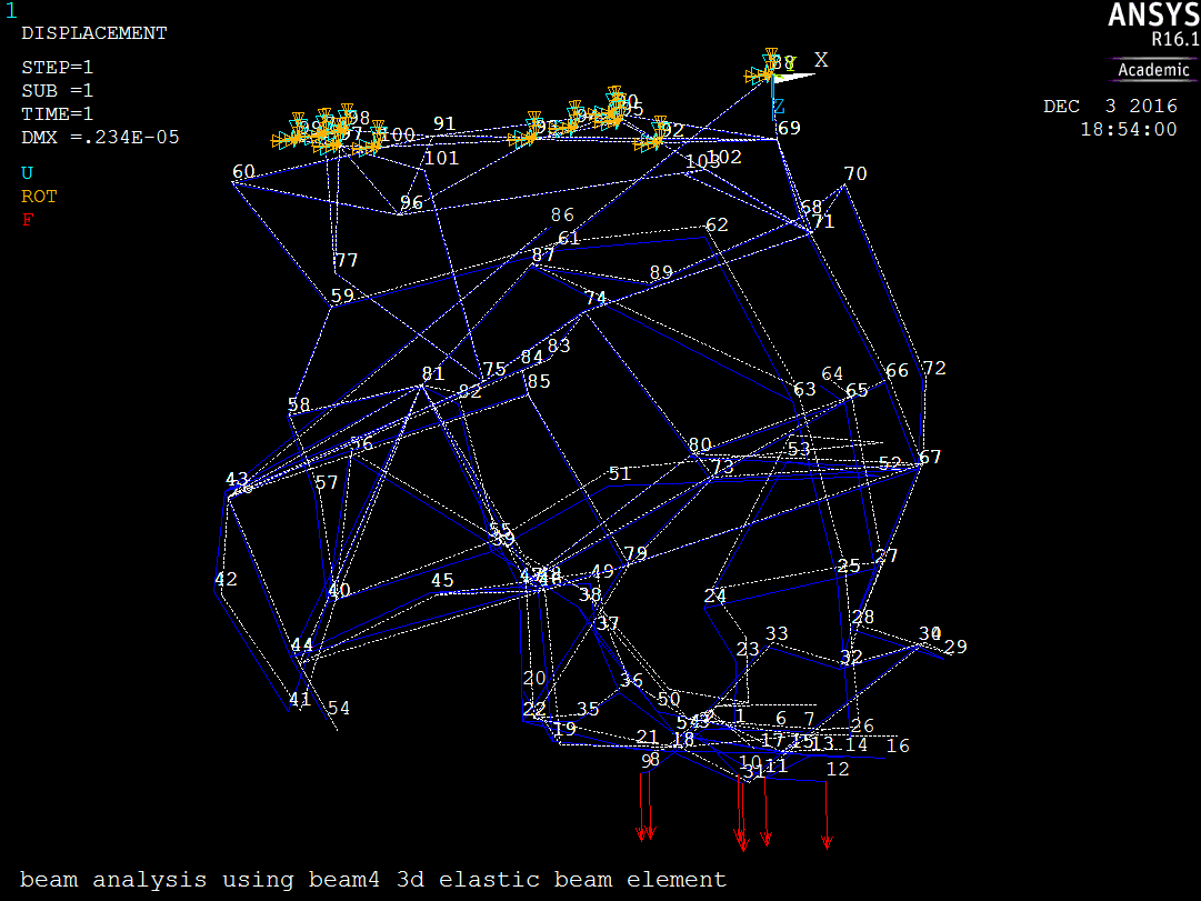
The average z-displacement of all positive z-plane nodes was

$$\eqalign{ \bar{u}_z &=& (1.3749 + 1.3799 + 1.5337 + 1.5812 + 2.0301 + 0.07753)/6 \\ &=& 1.3296\times 10^{−6}~\text{m.}}$$

Strain was $\epsilon_z = \frac{1.3296}{50.48} = 2.6338\times 10^{−2}.$

Stress was $\sigma_z = \frac{1\times 10^{-9}}{(48.46\times 10^{-6})(48.46\times 10^{-6})} = 0.4258~\text{Pa.}$

The Young’s modulus was $E_z = \frac{\sigma_z}{\epsilon_z} = 16.17~\text{Pa.}$

Discussion

Table 2 summarises the Young’s moduli simulated in this project.

Ex (Pa)	Ey (Pa)	Ez (Pa)
113.5	109.1	16.17

Table 2: Simulated Young's moduli.

All three moduli fell within the empirically determined range of 0.1–1500 MPa, giving confidence to my simulated results. That said, as mentioned in the Theory, my model gives lower bound estimates; it is possible that the true Young’s moduli exceed this empirical range.

More notably, E_x and E_y matched each other closely, with a percentage difference of only $\begin{equation}\frac{113.5-109.1}{109.1}\times 100\% = 4\% \end{equation}$.

One of the assumptions made about the fibrin clot is that the clot is homogeneous and isotropic. Ideally, this means E_x = E_y = E_z; since the clot I modelled is only a small cubic sample out of a much larger clot, had the entire clot been simulated, any effects caused by the presence of local non-uniformities will likely be averaged out, and all three moduli should match each other more closely. The fact that with such a small sample, E_x and E_y already agree with each other to within 4% lends support to the assumption about the clot’s isotropy.

E_z on the other hand deviated significantly from either of the other two Young’s moduli. It had a percentage difference from E_x of

$$\begin{equation*}\frac{113.5-16.17}{113.5}\times 100\% = 86\% \end{equation*}$$

and from E_y of

$$\begin{equation*}\frac{109.1-16.17}{109.1}\times 100\% = 85\% \end{equation*}.$$

There are two possible explanations—which are not mutually exclusive—for this discrepancy. The actual fibrin clot was fabricated by injecting a mixture of chemical ingredients rapidly into a chamber mounted on a microscope slide. The chamber is much thinner than it is wide (see figure 10), and since the clot forms after the requisite mixture has been injected into the chamber, the shape of the chamber might have affected the fibrin network structure, causing it to become anisotropic along the thickness of the clot, i.e. in the z-direction.

Figure 10: Schematic of microscope slide used to fabricate the clot.

The other possibility stems from the way the clot was imaged under the microscope. The confocal microscope took thin optical sections through the z-depth of the sample. These sections were subsequently stacked and combined to form a 3D reconstruction of the clot. Thus the vertical resolution of the scan could not be perfectly matched with the resolution in the plane of each optical section (the xy-plane). This resulted in noticeable smearing of clot structure in the xy-plane that was visible in the 3D printed model as thick clumps of fibrils in the z-direction.

In any case, in my model more fibrils may consequently have been oriented in the xy-plane than along the z-axis. The axial rigidity of a fibrin fibril is defined as

$$\begin{equation*} AE = \pi \left(\frac{1.154\times 10^{-6}}{2}\right)^2(5\times 10^{6})=5.23\times 10^{-6}~\text{N,}\end{equation*}$$

while its flexural rigidity is defined as

$$\begin{equation*} EI = (5\times 10^{6})\left(\frac{1}{4}\right)\pi\left(\frac{1.154\times 10^{-6}}{2}\right)^4=(4.35\times 10^{-19})~\mathrm{N\cdot m^2.}\end{equation*}$$

Since $AE\gg EI$, fibrin fibrils are much stiffer when loaded axially than when undergoing bending. If fibrils lie predominantly in the xy-plane, the clot would resist loading in the x and y directions—where most fibrils are loaded axially, than in the Z direction—where most fibrils are loaded flexurally. The combined effect of these factors may have caused the almost 90% deviation we saw of E_z from either E_x or E_y.

Of perhaps greater interest is the dramatic difference between the bulk Young’s moduli of the clot, which were on the order of 100 Pa, and the Young’s modulus of an individual fibrin fibril, 5 MPa as used in my simulations.

This phenomenon can be understood in terms of conformational changes in the fibrin network as loads are applied to it. The spring analogy in figure 11, where springs connected in a combined series and parallel configuration represent a network of fibrin fibrils of Young’s modulus $E$, demonstrates that the total elongation of a network of fibrils can be achieved with little or even negative strain in individual fibrils. Depending on the actual arrangement of fibrils, the network may have a much lower overall stiffness than a single fibril.

Figure 11: Spring analogy for conformational change in fibrin network.

In addition, Bradshaw et al. [8] showed that fibrin and similar proteins can even undergo conformational changes at the molecular level due to external loading, which may contribute to the elongation of networks of fibrils and the capacity of these networks for large strains.

Empirical analyses [9, 10] of the protein fibronectin have hinted that molecular conformational changes may arise from molecular rearrangement of fibrils, as well as protein unfolding of individual fibrils. A similar mechanism may be at work in fibrin.

My simulations cannot capture these molecular factors. They do show, however, that molecular structural modifications induced by external forces may further reduce the overall stiffness of the fibrin network relative to single fibrils, and underscore the inadequacy of any analysis of a fibrin clot based purely on a macroscopic solid mechanical model.

Conclusion

This complex procedure to model a fibrin blood clot, from imaging the clot, to slicing it optically, to 3D printing it, mapping nodal coordinates, then simulating its deflection in ANSYS, has proven to be a useful tool for performing stress and strain analysis on the clot. In order to apply this method to larger, denser, more complex clots though, the procedure must be adapted to automate node generation, which even with such a small and porous clot was very labour intensive and time-consuming.

References

[1] ANSYS, 2016. “ANSYS Academic Research, Release 17.2, Help System, Beam4 3d Elastic Beam”. ANSYS, Inc.

[2] Weisel, J. W., 2004. “The mechanical properties of fibrin for basic scientists and clinicians”. Biophys. Chem., 112(2-3), Dec., pp. 267–276.

[3] Lawrence, K. L., and ANSYS, I., 2007. Ansys tutorial: Release 11.0. SDC Publications, Mission, KS. OCLC: 166390730.

[4] Beer, F. P., ed., 2011. Mechanics of materials, 6th ed. McGraw-Hill, New York.

[5] Guthold, M., Liu, W., Sparks, E. A., Jawerth, L. M., Peng, L., Falvo, M., Superfine, R., Hantgan, R. R., and Lord, S. T., 2007. “A Comparison of the Mechanical and Structural Properties of Fibrin Fibers with Other Protein Fibers”. Cell Biochem. Biophys., 49(3), Oct., pp. 165–181.

[6] Wufsus, A., Rana, K., Brown, A., Dorgan, J., Liberatore, M., and Neeves, K., 2015. “Elastic Behavior and Platelet Retraction in Low- and High-Density Fibrin Gels”. Biophys. J., 108(1), Jan., pp. 173–183.

[7] Schindelin, J., Arganda-Carreras, I., Frise, E., Kaynig, V., Longair, M., Pietzsch, T., Preibisch, S., Rueden, C., Saalfeld, S., Schmid, B., Tinevez, J.-Y., White, D. J., Hartenstein, V., Eliceiri, K., Tomancak, P., and Cardona, A., 2012. “Fiji: an open-source platform for biological-image analysis”. Nat. Methods, 9(7), June, pp. 676–682.

[8] Bradshaw, M. J., Cheung, M. C., Ehrlich, D. J., and Smith, M. L., 2012. “Using Molecular Mechanics to Predict Bulk Material Properties of Fibronectin Fibers”. PLoS Comput. Biol., 8(12), Dec., p. e1002845.

[9] Bradshaw, M., and Smith, M., 2011. “Contribution of Unfolding and Intermolecular Architecture to Fibronectin Fiber Extensibility”. Biophys. J., 101(7), Oct., pp. 1740–1748.

[10] Smith, M. L., Gourdon, D., Little, W. C., Kubow, K. E., Eguiluz, R. A., Luna-Morris, S., and Vogel, V., 2007. “Force-Induced Unfolding of Fibronectin in the Extracellular Matrix of Living Cells”. PLoS Biol., 5(10), Oct., p. e268.

Acknowledgements

I would like to thank Professor Siddiqui and Professor Everbach for their mentorship, support and advice throughout the course of this project. In addition, I would like to thank Professor Vallen in the Biology department for training me to use the confocal microscope, as well as Irina Chernysh in the Department of Cell and Developmental Biology at the University of Pennsylvania for sharing her recipe for making fibrin with me.

Appendices

Appendix A

The ANSYS input .txt file used to run all simulations in ANSYS can be downloaded here.

Appendix B

The ANSYS output .txt file containing nodal displacements u_x, u_y and u_z can be downloaded here.