Numerically solving Rayleigh-Plesset in Mathematica

Luke Barbano, a fellow Swarthmore student who previously worked under the guidance of Professor Carr Everbach, laid the groundwork for the results of my post. His goal was to simulate the radial oscillation of a single bubble when subjected to a sinusoidal ultrasound field. Though his results did not quite match literature, it was an essential part of modelling sonothrombolysis. The holy grail of any research, as Carr put it, is to reproduce the same results empirically, analytically, and numerically. If one achieves that, the problem is considered fully understood and solved; time to move on to the next enterprise, to uncharted waters. The enterprise I have been tasked with however, is much less ambitious: model ultrasound- and microbubble-assisted clot dissolution numerically.

Two sides of the same coin: modelling a blood clot numerically—relative to which my E59 project is but a droplet in a haemal ocean; and modelling microbubbles numerically. Luke’s work is the basis for the latter.

The summer one year prior, I made some ad hoc changes to Luke’s Matlab and Mathematica scripts but still failed to replicate literature results. Carr suggested, rather than hacking away at the same code, that I start afresh. I returned to The Acoustic Bubble (Leighton, 1994) and transferred the Rayleigh-Plesset equation

$\begin{equation*} R\ddot{R}+\frac{3\dot{R}^2}{2} = \frac{1}{\rho}\left\{ \left( p_0+\frac{2\sigma}{R_0}-p_v \right)\left( \frac{R_0}{R} \right)^{3\kappa}+p_v-\frac{2\sigma}{R}-\frac{4\eta\dot{R}}{R}-p_0-P(t) \right\}. \end{equation*}$

into a Mathematica script, shown below. Note η is the dynamic viscosity, usually written as μ. P(t) is the driving sound field.

Clear[R, R0, \[Rho], P0, \[Sigma], Pv, \[Eta], P, \[Kappa]]
(*initial radius 2mm*)
R0 := 0.002
(*density of water 1000 kg/m^3*)
\[Rho] := 1000
(*static pressure 101325 Pa*)
P0 := 101325
(*surface tension of water 0.07286 N/m; source: "Surface-tension values" Wikipedia*)
\[Sigma] := 0.07286
(*Vapour pressure of water 2338.8 Pa*)
Pv := 2338.8
(*Shear or dynamic viscosity of water 0.001002 Pa-s*)
\[Eta] := 0.001002
(*10kHz sound field of pressure amplitude 2.7 bar*)

P[t] := 270000*Sin[2*\[Pi]*10000*t]
(*Polytropic index 1.4 since adiabatic*)
\[Kappa] := 1.4
NDSolve[{R[t]*R''[t] + (3 (R'[t])^2)/2 ==
   1/\[Rho]*((P0 + (2*\[Sigma])/R0 - Pv)*(R0/R[t])^(3*\[Kappa]) +
      Pv - (2*\[Sigma])/R[t] - (4*\[Eta]*R'[t])/R[t] - P0 - P[t]),
  R[0] == R0, R'[0] == 0}, R, {t, 0, 0.001}]
Plot[Evaluate[R[t] /. %], {t, 0, 0.001},
 AxesLabel -> {"Time (s)", "Bubble radius R (m)"}]

Apologies for the absence of syntax highlighting; Rouge currently does not support the Wolfram language of Mathematica—a massive oversight in my opinion.

Here’s the output:

Rayleigh

Figure 1: A bubble of radius 2mm, subjected to a 10kHz sinusoidal sound field of amplitude 270,000Pa.

Figure 1 matches figure 4.6 in Leighton exactly; a very encouraging sign.

LeightonFig4_6

Figure 4.6, pp. 309, The Acoustic Bubble by T.G. Leighton, 1994.

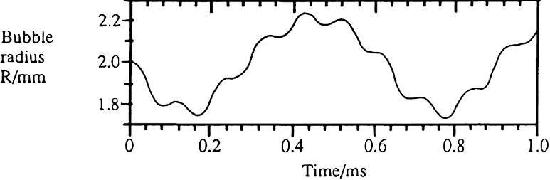
The bubble behaviour in figures 1 and 4.6 are largely periodic. I ran an additional check for a bubble slightly below resonance size. If my script correctly predicts the much more chaotic oscillations one would expect that match Leighton’s figure 4.7, I feel confident I have implemented Rayleigh-Plesset correctly.

LeightonFig4_7

Figure 4.7, pp. 309, The Acoustic Bubble by T.G. Leighton, 1994. Bubble radius 0.10mm subjected to a 10kHz sinusoidal sound field of amplitude 240,000Pa.

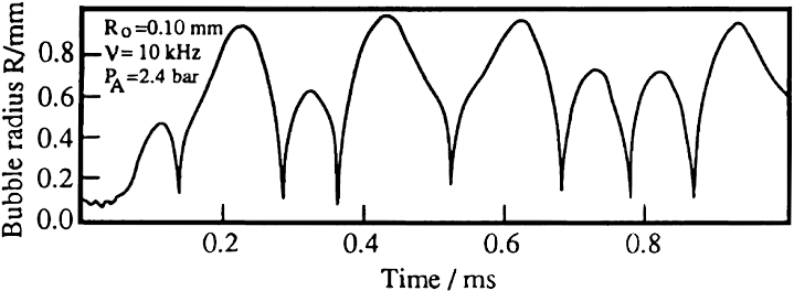
The result is decidedly unexpected.

RayleighResonance

Figure 2: A bubble of radius 0.1mm, subjected to a 10kHz sinusoidal sound field of amplitude 240,000Pa.

Notice that if I lower the pressure amplitude ever so slightly, from 240,000Pa to 239,120Pa, the radius-time curve is noticeably altered, matching figure 4.7 in Leighton.

RayleighResonanceAdjusted

Figure 3: A bubble of radius 0.1mm, subjected to a 10kHz sinusoidal sound field of amplitude 239,120Pa.

In retrospect, the fact that the bubble is near resonance size means small changes in inputs are amplified by the chaotic response of the bubble, reminding me of the logistic map. Leighton expresses a similar sentiment on page 311: “a small change in certain parameters ( $P_A$ , $R_0$ , $\omega$ ) could bring about a dramatic change in the radius-time curve.” (pp. 311, Leighton, 1994) There are many constants present in the Rayleigh-Plesset equation that undoubtedly play a role in its solution as well. Since Leighton does not specify what values he used, it is not unreasonable that our pressure amplitudes are somewhat different.

I wanted to see whether over a longer time scale the transient response might die out, leaving behind only the stable, periodic response. Increasing t tenfold from 0—0.001s to 0—0.01s immediately saw Mathematica throwing up its hands and throwing me a singularity or stiffness error. Fearing the latter, I wanted to switch to a stiff solver, only to discover Mathematica usually takes care of it automatically. Singularity then.

I reduced t to just beyond the location of the suspected singularity at 0.00123s, and voilà! the radius goes to negative infinity.

rayleighResonanceSingularity

Figure 4: Infinite negative radius... Delicious. Inertial cavitation posing as stable cavitation.

Evidently the bubble is unstable; it just took a bit longer to collapse.

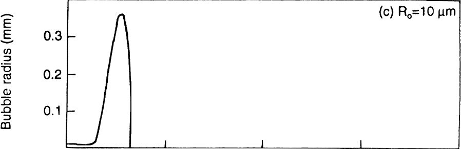
Suppose we make the bubble much smaller, down to microns, as characteristic of microbubbles?

rayleighInertial

Figure 5: Inertial cavitation experienced by a bubble of radius 10μm, i.e. the radius of a typical microbubble. Notice the rapid collapse.

This matches Leighton’s radius-time curve.

rayleighInertial

Figure 4.8, pp. 310, The Acoustic Bubble by T.G. Leighton, 1994. Bubble radius 10μm subjected to a 10kHz sinusoidal sound field of amplitude 240,000Pa.

Carr provided a set of typical parameters one might encounter in realistic ultrasonic microbubble experiments:

Amplitude (zero to max): 500kPa to 2MPa
Frequency: 1.0MHz
Pulse length: 5μs (5 cycles per burst)
Bubble radius: 3.0μm, but perhaps start at 2.0μm and walk up to 3.5μm in steps of 0.1μm for 500kPa amplitude to find the resonance radius.

Here’s my Mathematica script:

Clear[R, R0, \[Rho], P0, \[Sigma], Pv, \[Eta], P, \[Kappa], sol]
(*initial radius 3\[Mu]m*)
R0 := 0.000003
(*density of water 1000 kg/m^3*)
\[Rho] := 1000
(*static pressure 101325 Pa*)
P0 := 101325
(*surface tension of water 0.07286 N/m; source: "Surface-tension values" Wikipedia*)
\[Sigma] := 0.07286
(*Vapour pressure of water 2338.8 Pa*)
Pv := 2338.8
(*Shear or dynamic viscosity of water 0.001002 Pa-s*)
\[Eta] := 0.001002
(*10kHz sound field of pressure amplitude 2.4 bar; also try 2.3912 bar. Pulse switches off after 5\[Mu]s.*)

P[t] := Piecewise[{{500000*Sin[2*\[Pi]*1000000*t], t < 0.000005}, {0, t >= 0.000005}}]
(*Polytropic index 1.4 since adiabatic*)
\[Kappa] := 1.4
sol = NDSolve[{R[t]*R''[t] + (3 (R'[t])^2)/2 ==
    1/\[Rho]*((P0 + (2*\[Sigma])/R0 - Pv)*(R0/R[t])^(3*\[Kappa]) +
       Pv - (2*\[Sigma])/R[t] - (4*\[Eta]*R'[t])/R[t] - P0 - P[t]),
   R[0] == R0, R'[0] == 0}, R, {t, 0, 0.00002}]
Plot[Evaluate[R[t]*1000000 /. sol], {t, 0, 0.00002},
 AxesLabel -> {"Time (s)", "Bubble radius (\[Mu]m)"}]
NMaximize[{Evaluate[R[t]/R0 /. sol[[1]]], 0 <= t <= 0.000005}, t]

The Piecewise function is used to ‘switch-off’ the sound pulse after 5μs. Not sure why [[1]] in the last line is necessary, though it probably has to do with ensuring dimensions match—perhaps sol is not a scalar.

Once I recorded $R_{max}/R_0$ for $R_0$ from 2.0 to 3.5μm, I turned to Python (in hindsight Mathematica could gladly have done it) to find the resonance size.

# import numpy library
import numpy as np
# set up and import matplotlib
%matplotlib inline
import matplotlib.pyplot as mp
# import seaborn library
import seaborn

# equilibrium radii
R0 = [2,2.1,2.2,2.3,2.4,2.5,2.6,2.7,2.8,2.9,3.0,3.1,3.2,3.3,3.4,3.5]

# maximum relative radius Rmax/R0
RmaxRel = [7.93585,7.55434,7.15335,6.69714,6.18627,5.73354,5.43936,6.38532,6.61822,6.51025,6.21851,5.7339,5.03286,4.22899,4.1211,4.00593]

# plot shifted H1 and L1 data in time domain
mp.plot(R0,RmaxRel)
mp.xlabel('Equilibrium radius $R_0$ ($\mu$m)')
mp.ylabel('Relative maximum radius $R_{max}/R_0$')
mp.savefig('findResonanceRadius.pdf')
mp.show()

Thankfully Rouge supports syntax-highlighting Python beautifully.

findResonanceRadius

Figure 6: R_max/R₀ is maximised at R₀ = 2.8μm. At this equilibrium radius, R_max/R₀ = 6.61822.

That is very close to 3.0μm, suggesting that 3.0μm bubbles are indeed amongst the ones that cavitate most violently in experiments. That said, strange, very large radial expansions are observed for $R_0\leq2.6$ . No idea why that happens—I must clear this with Carr before finalising my slideshow for ASA Boston.